Gang Fang's Blog

lec3 model reproduction and experimentations: https://github.com/gangfang/makemore/blob/main/makemore_mlp.ipynb

Implementation notes:

• A good way to understand the training, val and test splits is that training split is used to train the params, val split is used to “train” the hyperparameters and test split is used to evaluate the trained model. The test split is used very sparsely, otherwise, we risk overfitting the test split.
• The way to create the train/val/test splits: my splitting solution is to divide the original dataset derived from the word list but i can’t do this because 1) the word list is not random and 2) the possibility of examples of certain pattern like the beginning of a word e.g., [“.”, “.”, “.”] congregating should be avoided. Therefore, we should split the word list instead of the original dataset
• (ChatGPT) General Guidelines on batch size:
  • Small to Medium Datasets: (like yours with 200,000 samples): Batch sizes of 32, 64, or 128 are common starting points.
  • Larger Batch Sizes: (256, 512, or even higher) can be used if your hardware supports it, potentially leading to faster training times due to better hardware utilization. However, very large batch sizes may require adjustments to the learning rate and other hyperparameters to maintain model performance.
• When I run predictions or sampling after training, the focus should be data transformations around the input to the model and the output from the model. “Model” simply refers to a forward pass.
  • numbers in, numbers out
• Init of all params uses torch.randn(), which gives me a standard normal distribution
• C[X]: what this is really doing is the addition of C.dim()-1 more dimension to X.dim()
• emb.view(-1, 30).dim() is determined by the number of params in .view(...)
• logits[0], obtained from a 27-neuron output layer, looks like this: tensor([ 3.3478, 1.8774, -6.6540, -0.2367, 3.2826, 1.3549, -10.8064, -0.4364, -6.1436, 2.8120, -4.2208, -1.2841, -0.9767, -4.0530, 1.7604, 0.5837, -8.4227, -9.8610, -3.4483, -2.1074, 0.4508, -2.1243, -1.3341, -4.0586, -14.1111, 1.7395, -0.7511]. This gets turned into a prob by softmax.​​​ (Softmax formula) This is then used to:
  • compute the loss value, which is a scalar
  • sample or make predictions
• Different init schemes for lec2’s model:
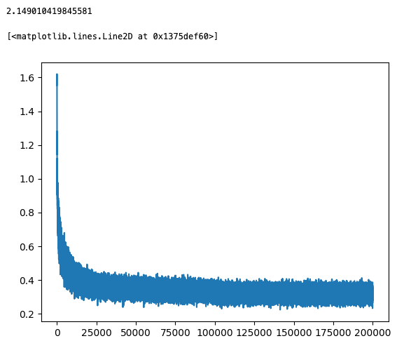
  • randn(): the initial loss is bigger. The beginning phase of the training (i.e., the first 100 iterations) drastically reduces the loss down to less than 5. The following phase is a slow, very slow, but steady reduction of the loss.
  • rand(): the initial loss is smaller, around 10. Then the loss fluctuates greatly, between 2 and 10, and then suddenly reduces its fluctuation to a much more desirable and smaller range, like 2 and 3.
• How do I explain the the difference in the initial loss with the two different initialization methods? How do I explain the weird optimization process with rand()?
  • one hypothesis for the diff initial losses is the default randn() returns a standard normal dist, which has a wider range than rand().
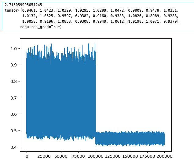
  • I just ran an experiment with [-2, 2] uniform dist using rand(), and the optimization process looks a lot more like the one with randn(). The initial loss is bigger, which provides confidence for the above hypothesis and the steady decrease of the loss makes me think including negative values in the initial params might be what makes the different. – SELF CORRECTION: nope, it has nothing to do with whether negative values are used in init. When I used [0.1, 0.3], I was able to get a pretty good loss at the end of training and params in the trained network contain negative values, which they should be. And the reason should be there are enough values that are near 0 so that the value of a lot of activations starts out on the slope of tanh resulting in a more effective gradient descent (v.s. they start out in the range where tanh is saturated and flat, which makes learning very slow). – CONFIRMATION: the above is correct, I ran one with [-4, 0] range and I got basically the same graph, the one that looks weird.
  • I am also seeing the sudden shift of the range of loss value when only positive values are used for init occurs at the iteration where learning rate drops from 0.1 to 0.01. – UNDERSTANDING: it’s not that the process suddenly enters a better phase but the minimization of the learning rate simply brings down how far the loss can jump from one iteration to the next, which results in a smaller range of fluctuation.
• Can optimization still work when all params are initialized to a single value, like 1? – AN: yes for like logistic regression. nope for neural networks due to symmetry of computational pathways in the ann.
  • when I initialized all params to closer to 1, the loss couldn’t get lower than about 2.8. And there is a big difference between a loss of 2.8 and a loss of let say 2.1. With a loss of 2.1, the params occupy a much larger range of value, what I saw is -1.5 to 1.7. With a loss of 2.8, the range basically stayed at 1.

• RNN as a universal approximator but not very trainable with the first order gradient based technique. We will see why it’s hard to train by looking at the activations and gradients. Models that come after RNN are designed to improve on trainability.
• All the nll we have been doing is conditional, and not unconditional (i.e., introduced in section 5.5 of theory book) because label Y is involved. However, in the bigram counting approach, we made ourselves god by counting all possibilities, therefore knowing the underlying distribution p_data. The trick is we made the problem so narrow (i.e., bigram) that all possibilities can be counted, which renders any estimation unnecessary.
  • this conditional log likelihood estimator also underlies all current LLMs because these models are trained to predict the next word in a sequence given the previous words, which is a conditional probability P(next word | previous words;θ).
  • and this connects back to my system 2 AI study: the training of world model is to maximize P(X;θ) while these LLMs maximize P(Y|X;θ). (ML street talk video)
• A thing about softmax: the purpose of the exponential function, from the perspective of a statistical language model, is to convert the logits into “soft counts”, something that can be normalized, just like real counts, to get the probability distribution. What the exponential function really does is to turn all logits positive and amplify difference between logits.
  • Only one thing to remember about logits: they are the raw outputs of the output layer before an activation function, like softmax, is applied. And they represent unnormalized log probabilities. This interpretation of logits is derived from walking backward from what the results of softmax represent, which are probabilities.
• “E04: we saw that our 1-hot vectors merely select a row of W, so producing these vectors explicitly feels wasteful. Can you delete our use of F.one_hot in favor of simply indexing into rows of W?” – AN: yes, and the use of embedding in Bengio’s 2003 paper feels just like this. GPT-CONFIRMATION: “When you use an embedding layer, you essentially skip the one-hot encoding step and directly index into a matrix of learned word vectors (the embedding matrix). This is more memory-efficient and allows the model to easily capture and leverage semantic relationships between words.”

High-level:

• Bengio’s AI scientist talk: he said ChatGPT making wrong answers confidently IS overfitting. how do i understand it? let’s break it down: “confidently” bit is easy, it refers to the model’s bias towards fluency. “Wrong answers” imply there is no guarantee of correctness in responses generated by the model. overfitting by my consideration is the model’s failure to faithfully estimate the empirical distribution defined by the training set. So what bengio said makes sense: the overfitted model using the spurious patterns it learned, due to it being more complex, to answer a question incorrectly and fluently.
  • wrong answers are rare, because most general questions asked to chatgpt are within the bound of the training set.
• On the debate of whether these LLMs have understandings, a important direction of thinking is to decide whether a model simply responses to a question by reproducing the example it saw during training, implying that question and answer pair is contained in training data, or it discovered abstractions or concepts during training and uses those discoveries to answer the question, implying this question is novel. As I was writing this some related thoughts came up:
  • this seems to be a matter of interpolation. I don’t think I need to doubt the basic ability of the model to generalize to unseen data (i.e., questions) and therefore to answer them successfully. Even with a reductionist view (i.e., emergent properties are ruled out of the discussion), knowing that a CNN does “see” patterns from the pixel up gives me confidence in saying these language models pick up some, I am being intentionally ambiguous here, more abstract information, which is used to respond to unseen queries within the space bounded by the entire training set. In a word, these models aren’t hash tables and they can generalize within the same distribution.
  • the more interesting case would be extrapolation, or ood generalization.
  • calling these models stochastic parrots isn’t wrong because these models are inherently probabilistic and they are built to mimic human language. But the thing that this analogy misses is the fact that these models do pick up patterns while animal parrots don’t, they aren’t even hash tables, they just repeat.
• Do the regularities or patterns in the training corpus captured by the LLMs the same thing as concepts, abstractions or even understandings?
• “AI scientist” is a much better term than AGI, in terms of formulation of the problem. AGI is too broad of a term, it can mean anything, which doesn’t provide concrete directions. But AI scientist restricts the scope of inquiry to designing and building models that are capable of performing scientific discoveries on their own, implying they understand the material world and are able to extrapolate and generate truly novel ideas.
  • He also provided a summary of the iterative discovery process in his talk. Now I think I understand more why those GFN people are working on drug discoveries, they use this new framework in practice.
• Some key ideas in Bengio’s new framework: diversity, Bayesian posteriors, which are computable, exploration rather than optimization.