Gang Fang's Blog

Updated on Jun 14, 2024

• we use a varying context length up to the block_size. This is to facilitate the transformer’s ability to predict the next character with context of different sizes. For example, if the block size is 8, then the transformer will be able to predict the next character using the previous one character or 2 … or 8 characters.
• Simpler models can take a larger learning rate like 1e-3. Usually 1e-4 is used for more advanced networks
• Using hardware to accelerate training
• F.cross_entropy() expects logits to be of form (minbatch, C, d1, d2, ..., dk). The channel dimension should be the second dimension
• Notice the difference between the organization of this data and that of makemore (i.e., name) data. The makemore data is simpler in that it consists of names, which structures the data with each name having an start and an end. A block, defined by the block_size, operates within a name. On the contrary, this shakespera data is a blob of text, there is no inherent structure to it and hence allows abitrary slicing. A block in this context operates in the entire text blob and the positioning of it is determined by a random process (i.e., randint()) since there is no natural start points.
  • WAIT, the above analysis doesn’t seem to be complete. Even though there is a natural start and end point of a name, the def build_dataset(words): function uses a block to slide through a word and repeats for all words. And the X in data contains examples of blocks instead of words. And then, I can use the same technique (i.e., block sliding) for the entire text blob in this data, producing a dataset of a size of (len(text) – block_size).
  • So I guess they are different options for setting up the data.
• why is my code using AdamW not optimizing the bigram model? AN: because I put zero_grad() before step(). Since .data -= lr * .grad, nothing happens when .grad is 0
• printing of matrix data: I only need to print one example when an individual example is the focus. Printing the entire data set makes it harder to reason
• what makes the bigram model bigram in terms of its training loop? AN: the answer lays in the targets and the construction of the logits from idx and. The data loader defines a target as simply the next character after the char in idx. So after I convert idx to logits using the embedding table and the subsequent .views, which is really a conversion of the time dimension into the batch dimension, what I get is the logits of one character and the corresponding target of that character, the next character. This whole process makes the model bigram.
  • self.position_embedding_table(torch.arange(T)) simply returns the weights of the emb table. When this position_embedding_table is used in the bigram model, we have awareness of the position of the char in the T dimension but under the context of a bigram, as in the block preceding a char is still not used by the model.
• Embedding explained by 3Bule1Brown (video): the directions in the high dimension space of the embedding can correspond with semantic meaning. An example is E(aunt) - E(uncle) ~= E(woman) - E(man)
• the feedforward layer after the multi-headed attention layer is applied to each individual token in the input sequence/block. Andrej said this is individual token doing the thinking after communicating with other tokens in a input sequence. Based on self.ffwd = FeedForward(n_embd) and x = self.ffwd(x) # (B,T,C), we see self.ffwd(x) works on all tokens in (B, T). There are B * T of them.
• three blocks of communication followed by computation is already considered deep by Andrej and he said this suffers from optimization issues. But there are two techniques to cope with the depth of the network:
  • residual connections
  • layernorm
• Kaiming He’s 3 contributions to deep net training: (this is his theme)
  • initialization
  • normalization
  • residual connections
• Andrew Ng: good performance on the training set it’s usually the prerequisite of good performance on the eval set or test set
• An identity function or identity operation is a function that returns its input without any change

Residual Networks (ResNets)

• Andrew Ng said called 100-layer network deep. But he said that 6 years ago. OK, so GPT3, trained 3 years ago, only has 96 layers. but the number of parameters, 175 billions, is probably a lot more than that of the 100–layer network 6 years ago.
• motivation of resnets: In theory, the deeper a neuron net, the better the training performance. however, in reality, at a certain point, the depth of a neuron net actually worsens the training performance because training simply gets harder and less effective. Residual network is designed to combat this problem.
• Structure of a residual block: it consists of a main path and a shortcut/skip connection. The main path and the shortcut run in parallel. They are added before the last non-linearity of the block.
  • C4W2L03 Resnets

Attention

• I understand the procedure of producing the self attention. but what are the intuitions behind the key and query and how are they achieved through the mathematical operations? Andrej said the intuition of the key is what a token can provide and that of the query is what a token is looking for. This makes some sense but not completely. I also know that the key and the query are learned. But this line wei = q @ k.transpose(-2, -1) can also be changed by swapping the position of q and k to get wei = k @ q.transpose(-2, -1) because k and q come from the exact same operation nn.Linear(...)
  • My response to the confusion: the meaning of k and q is assigned by data during training. So the computation doesn’t care what they are called (i.e., k and q). Their names are only useful to human who is reading and understanding their roles in the computation.
• 1B3B said masking is necessary because each block provides number of block size sub-examples for training. I think an easier way to understand masking is we simply use words coming before the query words as keys in training because we always predict the future words using the previous words.
• what attention really aims to do explained by 3Blue1Brown: (we simplify and assume words are tokens in this discussion)
  • refining the meaning of a polysemous word (i.e., a word with multiple meanings). Under the context of the embedding space, adjusting the direction of a word in the embedding space given its context.
    • note that the original direction of a polysemous word always has one direction.
  • more generally, moves information in the embedding of a word to that of another. Words can be far apart and more and more context is aggregated.
    
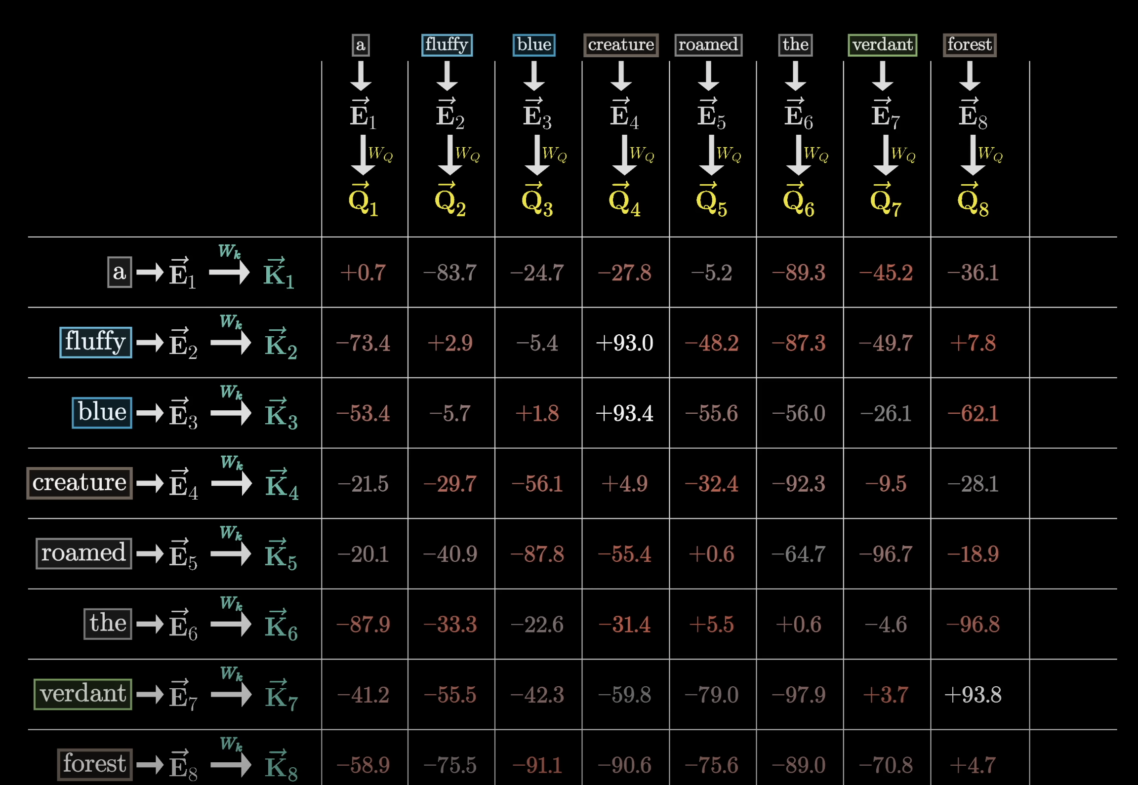
• In the above snapshot, we can see the dot product matrix showing how relevant each word is, based on the key, to the query of another word, and hence the update of meaning of that another word
  • And this is achieved by the matrix multiplication in Andrej’s lecture: wei = q @ k.transpose(-2, -1). The resulting T by T matrix shown as that in the snapshot is the attention pattern
  • the whole point of q @ k is to let every position in q meets every position in k and constructs the attention pattern, which is the result of every single interaction between q’s element and k’s element. Then training takes care of tuning the attention pattern so that the trained attention pattern tells us the degree of relationship between a q’s element and a k’s element.
• Back to the question I have in the first bullet, I think this is challenging to understand because a query is nothing but concrete. The example 1B3B gave (i.e., noun looking for adj) is nice but how come the model ends up coming up with these semantically meaningful queries? And why keys end up to be answers to those queries?
  • GPT’s AN: “As the model learns, it discovers patterns in the data and adjusts Q and K vectors to reflect these patterns. Over time, the queries and keys capture meaningful semantic information because this helps the model make accurate predictions.”
  • My understandings: this makes sense from a statistical perspective. The model has no intention to pair nouns and adjectives but rather the pairing was “discovered” during training by the model because of the semantical patterns inherent in the text/training data.
    
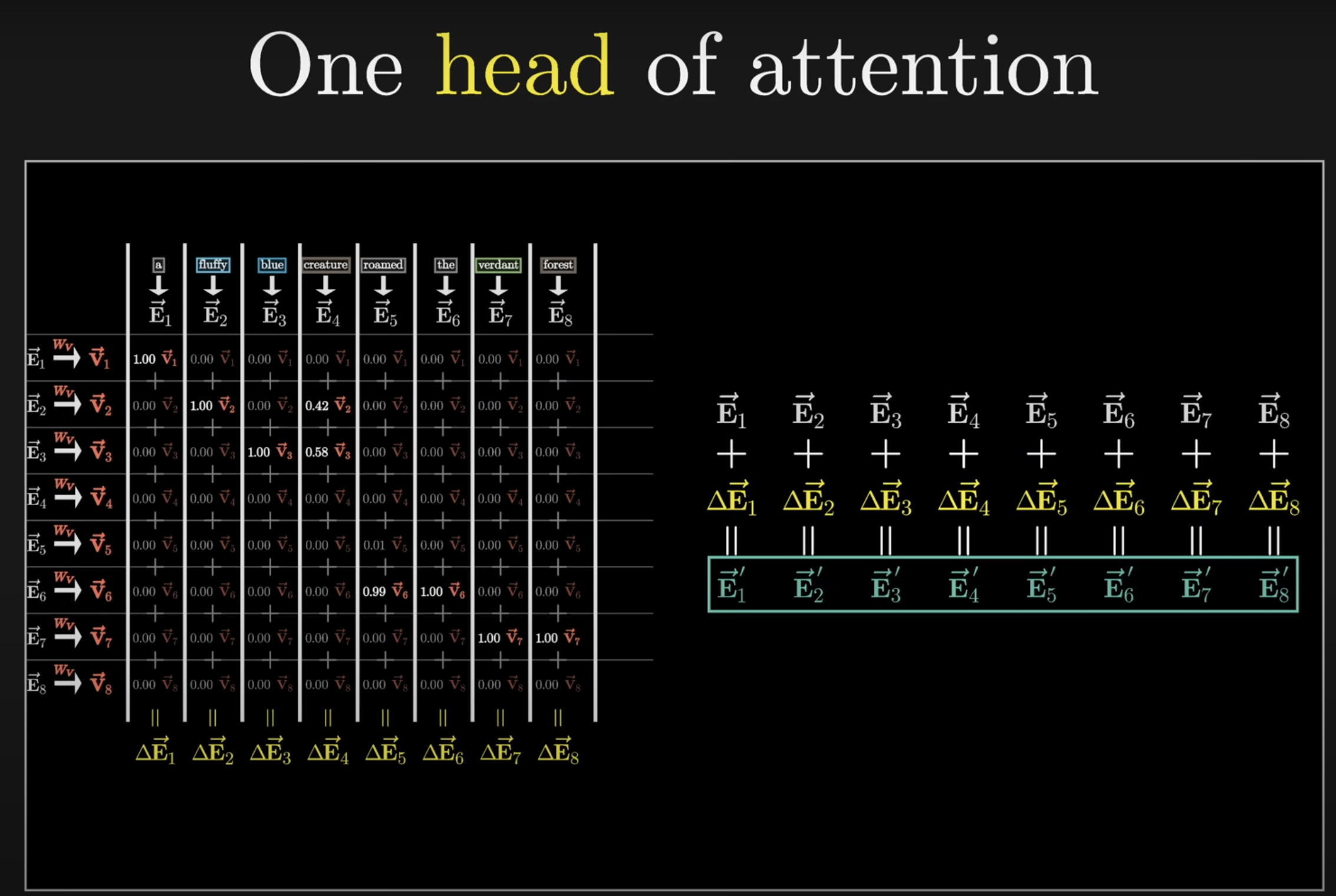
    (In 1b3b’s video, Wv is assumed to be square of size C by C.)
• The value matrix Wv discussed in the 1B3B video doesn’t seem to be the same as that in Andrej’s video v = value(x). How are they different? Analysis: out = wei @ v achieves the animation in 1b3b video that performs the weighted sums for all tokens’ embeddings, yielding the out of size (T by head_size). It seems to me the 1B3B’s value matrix corresponds to value = nn.Linear(C, head_size, bias=False) because they contain params to be updated. AN: that is correct. Andrej’s value and the 1b3b’s value matrix are the same thing. Andrej’s v is simply the collection of all value vectors of the input sequence.
  • in general, the value matrix has a size of (C, head_size). In 1b3b’s video, the value matrix is assumed to be square of size C by C.
  • the output of a single head of attention in a multi-headed design has the size of (block_size, head_size)
• The delta E1~8 in the snapshot obtained by the column-wise v vector summation is the same as Andrej’s out = wei @ v. wei is T by T and v is T by head_size (in the snapshot, head_size equals to C). The intuition of this matrix multiplication is a weighted sum of all elements of the same head index, in the sequence (e.g., v1_1, v2_1, v3_1… v8_1), which is then concatenated along the head dimension to yield delta E1~8 of size T head_size
• In a multi-headed attention mechanism, embedding_size = num_head * head_size. Such design makes sure when each head’s output vector is concatenated, the multi-headed output has the size of embedding_size, which allows for seamless integration into subsequent layers. Intuitively, the goal of the design is for each head to capture different features or aspects of the input data, combined to provide a comprehensive representation
• Multiple attention heads in each attention layer and multiple attention layers in a transformer arch.
  • multiple attention heads: they capture various types of relationship and dependencies (e.g., noun and adj pairing) in the data
  • multiple attention layers: More complex representations of input data are developed as it passes through the network.
• they intuition behind the query matrix, key matrix, and value matrix: query matrix and key matrix together enable data-based attention (i.e., the attention pattern grid). The value matrix facilitates the (semantic) adjustment of query token in the embedding space driven by the key tokens.
• Andrej’s 6 notes on attention:
  • Communication
  • no notion of space
  • independent within batch
  • encoder block vs. decoder block: a decoder block is a masked encoder block
  • self attention vs. cross attention
  • scaled softmax: in wei = q @ k.transpose(-2, -1) * head_size**-0.5 , head_size**-0.5 reduces the var of wei so that F.softmax(wei, dim=1) doesn’t turn into an one-hot vector, which is undesirable because the communication will become one on one