Gang Fang's Blog

Code reproduction of Andrej Karpathy’s “building makemore part 5” lecture: https://github.com/gangfang/makemore/blob/main/makemore_part5.ipynb

Study notes:

• continue pytorchifying the code:
  • generalize the layer list: adding in embedding layer and flatten layer to the list
  • use a model class (i.e., Sequential) to encapsulate all the layers and the forward pass operation
• seemingly small difference in loss means hugely in the sample outcomes for the model we built: with a loss of 3.5, the samples are complete gibberish while with a loss of 2.1, the model provides much more name-like results, even though they are not perfect.
• Why taking in all information in the first layer at once might be considered less effective compared to the dilated architecture used in WaveNet?
  • a reminder: the feature hierarchy I observed in CNNs performing image recognition comes from
  • Makemore_mlp vs. CNN: the linear layer in makemore_mlp is a fully connected layer. If I consider the first linear layer after embedding layer as the first layer, then the first layer takes in all information provided in the input (i.e., the context consisting of three characters), which makes sense given the small context length. Similarly, the first layer of a CNN takes in all information provided in the input also. However, the crucial difference occurs at the neuron level. Every neuron in the first layer of Makemore_mlp receives all information in the input whereas a neuron in the first layer (i.e., convolutional) in the CNN only receives information in its corresponding receptive field, defined by the conv filter.
  • receptive fields:
• Why is the embedding layer used? I wrote about the two interpretations of the embedding layer in this study note: it is either a matrix value retrieval or a matrix multiplication, depending on whether we view it through the lens of one hot encoding. I used one hot encoding in makemore.ipynb: # an ANN with one hidden layer; xenc = F.one_hot(xs, num_classes=27).float(); W = torch.randn((27, 27), requires_grad=True); logits = xenc @ W
  • what if I don’t use this one hot encoding here? AN: without one hot encoding, I am left with the scalar value as input. And that doesn’t seem to work with a layer in the neuron net because matrix multiplication cannot be performed.
  • how can I represent this embedding layer in a diagram? I can only do it with the one hot encoding interpretation mentioned above and it is a linear layer of 27 by 10 where the 27 input neurons will only have one neuron with the value of 1 while everything else is 0. Then we have 3 sets (a context size of 3) of this linear layers, not connected back to front, but put together in parallel to form a 81 (3×27) by 30 embedding layer.
  • related: the hand written digit recognition uses input that require note encoding because the binary-value array representation of an image naturally works with matrix multiplication
• PyTorch related:
  • torch.no_grad() related:
    • Why is context manager with torch.no_grad() used when the last layer’s weights are scaled down to 0.1? AN: because I don’t want this discrete scale-down operation during initialization to be a part of the computation graph used for backprop later. If it ends up in the computation graph, it will have an impact on the backward pass where these weights will receive gradients also scaled by 0.1, affecting everything coming before the scaling operation.
      • The rule of thumb is whenever I need to manipulate some part of the network for init or testing, do it under no_grad() context manager.
      • Another way to look at this scale-down operation is an addition of layer right after the layer whose weights are scaled. But instead of scaling the weights of that layer, I scale the outputs of that layer by the constant. So effectively we have a new layer of element-wise scaling with unadjustable params. We have other unadjustable layers like Tanh() and Flatten().
    • Using @torch.no_grad() for def split_loss(split): is to avoid constructing a computational graph for the forward pass. By default, PyTorch dynamically constructs a computational graph during a forward pass and what def split_loss(split): does essentially is to run a forward pass on training data (or eval data) to obtain a loss. So in order not to get a computational graph created, we use the annotator.
    • Note that there is a difference in the above 2 points: the above first point is about the definition of the computational graph, ie how the graph will look like. The second point is about the actual construction of the computational graph according to the definition. The constructed graph is then used to compute the gradients. But note that pytorch uses the define-by-run approach where the network is determined during the training as the actual calculation is performed
    • The computational graph’s lifecycle is bounded within a single forward and backward pass. But how this boundary is defined and followed? AN after GPT: assuming no other references pointing to the graph, loss.backward() makes the graph disposable once gradients calculation is completed. And what comes after loss.backward() (i.e., forward pass in the next iteration) constructs the computation graph anew. GPT convo
  • torch.nn provides layers, activation functions, loss functions, utilities, and containers. It is a neural network library on top of torch.tensor
  • Container modules like nn.Sequential put together a list of layers to construct a model.
  • Matrix multiplication a @ b only works on the last dimension of a, the dimensions before the last don’t change
  • pytorch doesn’t have good documentation
• after FlattenConsecutive() transforms Embedding tensor (4, 8, 10) into FlattenConsecutive tensor (4, 4, 20), does the first Linear layer(fan_in: 20, fan_out: 200) only work on the last slice in the second dimension of the tensor [:, -1, :]? Based on the arch of wavenet below, it should. But I don’t think the code does, so I am confused.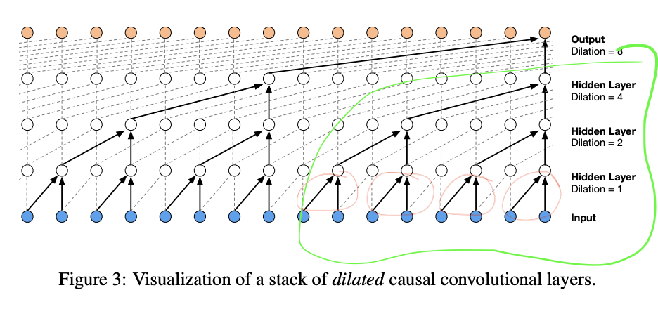
  • x (4 4 20) @ w (20 200) produces a tensor of (4 4 200) so apparently the linear layer applies to all 16 20-scalar long vectors (i.e., all 16 (4 times 4) vectors of size 20 multiplied by w and transformed into a new vector of size 200) and w is shared by all 4 circled in red. So is it still a wavenet??
    • This arch reuses params in a linear layer and this is why it’s CONVOLUTIONAL, same idea as that in CNN for images. An alternative arch is to use 4 set of params (no reuses) for the 4 red circles, each set for a circle.
      • Jun 1’s note: Is this really convolutional? “convolutional” is used to describe something that performs the convolution operation. The convolution operation is performed between two vectors where the reversed second vector slides along and dot product with the first from left to right to produce a third vector. The important thing here is it describes the whole sliding dot product process. In the context of CNN, that means a convolution operation only completes when a filter finishes sliding through the entire image.
      • The reversal happened to the second vector is motivated by the idea to only sum the multiplications of values of index summing to a certain value. An example is the second element of the resulting vector of convolute(v1, v2) (v1 and v2 both have 6 elements) is v1_1 * v2_2 + v1_2 * v2_1. Note that in each multiplication term, the indexes add up to 3.
      • And the point of CNN is to learn the kernel parameters. Since convolution is a fundamental math operation, different kernels are used to achieve different image processing goals. The power of CNN is that the kernel can be learnt based on the training data.
      • AN: therefore, the reuse of params in the linear layer itself is NOT CONVOLUTIONAL. It’s merely a component necessary for the convolution operation.
      • But what is a convolution?
  • Yes, Andrej said the code he presented implemented the green circled part of the arch with a context length of 8.
  • MY THINKING: it seems that I misunderstood the architecture of a wave net. Based on the diagram, the first layer does apply to all of input, but importantly in the grouped manner: if I only look at one example in the batch, the first linear layer is applied to all four vectors of size 20 at the same time independently and the receptive field size of this linear layer is 1/4 of the total input. Then all of them are transformed into a vector of size 200 because the Linear layer has a 20 fan_in and 200 fan_out. The next FlattenConsecutive layer further groups the tensor and transforms it from (4, 4, 200) into (4, 2, 400). And the following Linear layer therefore now has a receptive field size of half of the total input. The process repeats until the last linear layer “sees” everything in the input, dealing with a (4, 400) tensor.
• how should the batchnorm layer deal with the three dimensional tensor (4 4 200)?
  • MY GUESS: Batch norm is still here to normalize activation distributions, even in this new architecture. Given this principle, I think the transformation should be from (4 4 200) to (1 4 200)
  • ANSWER: my guess is wrong. The consistency across activation distributions should not only occur across batch, but also across spatial features (considering a neuron as a feature here). The way to think about this is to not look at the normalization at each group/filter but to look at it on a layer level. I want to make sure the mean and var calculated accounts for everything that happens in the layer, not just a group in the layer. This also enhances the stability of estimate of the mean and variance. See GPTs answer: https://chatgpt.com/share/18f9c398-84df-4b64-b22a-e54ac5dd9b81
  • Jun 1’s note:
    • remember that the ultimate goal of normalizations is to stabilize and speed up training
    • the reason why Andrej thinks normalizing only across batches and leaving out groups is a bug is because the running_mean and running_variance now have a shape of 1 4 68, which doesn’t make sense because the size of the hidden layer is 68 and we should only have one running_mean and one running_variance for each neuron.
    • my response: still, this is only a bug when we think at the layer level. If we want to normalize within each group, then it seems to me correct to have running mean and running variance for each group, even when there is only one set of parameters used for all the groups.
      I think the result Andrej himself got confirms my opinion. the validation loss he got after the “bug fix” is 2.022 while the prior one is 2.029. He said he wasn’t sure if this is of statistical significance. But he still expected an improvement because of the stability effect obtained by aggregating more data into the mean and var.
      
• Andrej’s dev process for deep nn:
  • spent a lot of time with the documentations
  • figure out all the shapes of tensors in the whole network
  • prototype in Jupiter notebook (i.e., to get the above done) and train in repo
  • experimental harness: set up evaluation harness, kick off experiments, a lot of arguments the script can take, look at a lot of plots of training and evaluation losses, search for hyper parameters
    • note that the process Andrej demonstrated in lecture is not a typical DNN dev process, which lacks experimental harness
• In the sampling code, if I use ix = torch.argmax(probs) instead of ix = torch.multinomial(probs, num_samples=1), the result would be: analissa. analissa. analissa. analissa. analissa. analissa. analissa. analissa. analissa. analissa.
  • This is because once the model is trained, it represents the prob dist. of the training data. To be precise, it represents 27 prob dist. for the 27 possible inputs (i.e., 26 chars and ‘.’), one dist. for each. So when ix = torch.argmax(probs) is used, a fixed outcome is guarenteed for a specific input. And since the start of a word is always the encoded ‘.’, the cascade of predictions and the resulting word are always the same. With the provided training data, that is analissa..
  • !!! A distinction can be made between sampling from a trained distribution, i.e., the neural network and the Bayesian approach, described by Yoshua Bengio. With the Bayesian approach, the sampling doesn’t happen after the training is done with a fixed probability distribution obtained by MLE. Instead, the sampling happens during the construction of the distribution. The outcome is that we will have multiple fixed distributions, i.e., neural networks, instead of just one.