One fundamental thing to remember is training examples occupy a dimension of the tensor manipulation.
When using jupyter notebook, it’s a good idea to random init of params in a separate cell so that reruns of subsequent operations won’t be affected by new initializations.
Cross entropy is a measure used in machine learning and statistics to quantify the difference between two probability distributions.
Why mini batch works so well (training effectiveness close to using full training set but much much better performance)? – AN: mini-batch finds us the approx. gradient each time an optimization step is run, and this approx. value is always so close to the actual gradient that the approx. value takes us to almost the same place in the loss landscape, while the computation of the approx. value is many times faster. This comes down to the marginal effect of optimization. We only want good enough and not perfect.
Training examples are a part of the computation graph of the loss. So we can see, with random mini-batches, loss of different iterations doesn’t always strictly descend. Sometimes the loss bounces up from the previous iteration’s loss because the current loss is measured by a different batch of training examples. This phenomonon is more pronounced when batch size is smaller. But the overall trend is certainly descending.
When finding the “decent” learning rate by plotting, it’s necessary to INCREASE the learning rate from lower bound as we iterate during training. But how should I make sense of it? Did I write something down in my 2015’s note about searching for a good learning rate? – AN: yes i did. In section 4.4, I wrote to find the best learning rate alpha we try out the number series 0.001, 0.003, 0.006 and so on all the way to the reasonable largest. And to answer the first question, how to make sense of it, I should not only look at the plot but also the set up: lre = torch.linspace(-5, 0, 1000); lrs = 10**lre gives a lower bound that is so small that training is basically ineffective as in training loss almost not decreasing in the plot and upper bound that is large enough that it creates overshots. With a plot set up in this way, we can see the trench is, not where the loss decreases the fastest, but where we can have the max learning rate GD can tolerate before the loss diverges. By identifying the trench and finding this max learning rate we make GD run as fast as possible.
Then a learning rate decay will follow
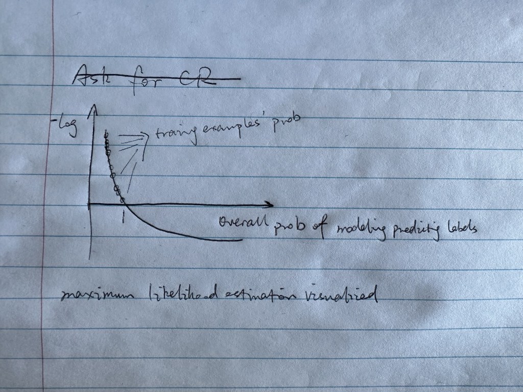
The essence of maximum likelihood estimation expressed in code and graph: loss = -prob[torch.arange(batch_size), Y].log().mean(). Graph is at the end of page.

Leave a comment